One of the most popular metrics in football analytics is the concept of ‘expected goals’ or xG for short. There are various flavours of expected goal models but the fundamental objective is to assess the quality of chances created or conceded by a team. The models are also routinely applied to assessing players using various techniques.
Michael Caley wrote a nice explanation of the what and the why of expected goals last month. Alternatively, you could check out this video by Daniel Altman for a summary of some of the potential applications of the metric.
I’ve been building my own expected goals model recently and I’ve been testing out a fundamental question regarding the performance of the model, namely:
How well does it predict goals?
Do expected goal models actually do what they say on the tin? This is a really fundamental and dumb question that hasn’t ever been particularly clear to me in relation to the public expected goal models that are available.
This is a key aspect, particularly if we want to make statements about prior over or under-performance and any anticipated changes in the future. Further to this, I’m going to talk about uncertainty and how that influences the statements that we can make regarding expected goals.
In this post, I’m going to describe the model and make some comparisons with a ‘naive’ baseline. In a second post, I’m going to look at uncertainties relating to expected goal models and how they may impact our interpretations of them.
The model
Before I go further, I should note that the initial development closely resembles the work done by Michael Caley and Martin Eastwood, who detailed their own expected goal methods here and here respectively.
I built the model using data from the Premier League from 2013/14 and 2014/15. For the analysis below, I’m just going to focus on non-penalty shots with the foot, so it includes both open-play and set piece shot situations. Mixing these will introduce some bias but we have to start somewhere. The data amounts to over 16,000 shots.
I’m only including distance from the centre of the goal in the first instance, which I calculated in a similar manner to Michael Caley in the link above as the distance from the goal line divided by the relative angle. I didn’t raise the relative angle to any power though.
I then calculate the probability of a goal being scored with the adjusted distance of each shot as the input; shots are deemed either successful (goal) or unsuccessful (no goal). Similarly to Martin Eastwood, I found that an exponential decay formula represented the data well. However, I found that there was a tendency towards under-predicting goals on average, so I included an offset in the regression. The equation I used is below:
xG = exp(-Distance/α) + β
Based on the dataset, the fit coefficients were 6.65 for α and 0.017 for β. Below is what this looks like graphically when I colour each shot by the probability of a goal being scored; shots from close to the goal line in central positions are far more likely to be scored than long distance shots or shots from narrow angles, which isn’t a new finding.

Expected goals based on shot location using data from the 2013/14 and 2014/15 Premier League seasons. Shots with the foot only.
So, now we have a pretty map and yet another expected goal model to add to the roughly 1,000,001 other models in existence.
Baseline
In the figure below, I’ve compared the expected goal totals with the actual goals. Most teams are close to the one-to-one line when comparing with goals for and against, although the overall tendency is for actual goals to exceed expected goals at the team level. When looking at goal difference, there is some cancellation for teams, with the correlation being tighter and the line of best fit passing through zero.
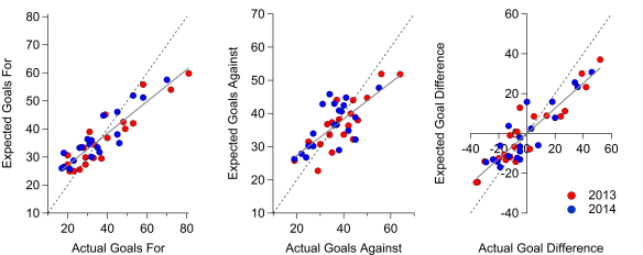
Expected goals vs actual goals for teams in the 2013/14 and 2014/15 Premier League. Dotted line is the 1:1 line, the solid line is the line of best fit. Click on the graph for an enlarged version.
Inspecting the plot more closely, we can see some bias in the expected goal number at the extreme ends; high-scoring teams tend to out-perform their expected goal total, while the reverse is true for low scoring teams. The same is also true for goals against, to some extent, although the general relationship is less strong than for goals for. Michael Caley noted a similar phenomenon here in relation to his xG model. Overall, it looks like just using location does a reasonable job.

The table above includes R2 and mean absolute error (MAE) values for each metric and compares them to a ‘naïve’ baseline where just the average conversion rate is used to calculate the xG values i.e. the location of the shot is ignored. The R2 value assesses the strength of the relationship between expected goals and goals, with values closer to one indicating a stronger link. Mean absolute error takes an average of the difference between the goals and expected goals; the lower the value the better. In all cases, including location improves the comparison. ‘Naïve’ xG difference is effectively Total Shot Difference as it assumes that all shots are equal.
What is interesting is that the correlations are stronger in both cases for goals for than goals against. This could be a fluke of the sample I’m using but the differences are quite large. There is more stratification in goals for than goals against, which likely helps improve the correlations. James Grayson noted here that there is more ‘luck’ or random variation in goals against than goals for.
How well does an xG model predict goals?
Broadly speaking, the central estimates of expected goals appear to be reasonably good. Even though there is some bias, the correlations and errors are encouraging. Adding location into an xG model clearly improves our ability to predict goals compared to a naïve baseline. This obviously isn’t a surprise but it is useful to quantify the improvements.
The model can certainly be improved though and I also want to quantify the uncertainties within the model, which will be the topic of my next post.
Pingback: Uncertain expectations | 2+2=11