A sumptuous passing move ends with the centre forward controlling an exquisite through-ball inside the penalty area before slotting the ball past the goalkeeper.
Rewind.
A sumptuous passing move ends with the centre forward controlling an exquisite through-ball inside the penalty area before the goalkeeper pulls off an incredible save.
Rewind.
A sumptuous passing move ends with the centre forward controlling an exquisite through-ball inside the penalty area before falling on his arse.

Source: Giphy
Rewind.
Events in football matches can take many turns that will affect the overall outcome, whether it be a single event, a match or season. In the above examples, the centre forward has received the ball in a super-position but what happens next varies drastically.
Were we to assess the striker or his team, traditional analysis would focus on the first example as goals are the currency of football. The second example would appeal to those familiar with football analytics, which has illustrated that the scoring of goals is a noisy endeavour that can be potentially misleading; focusing on shots and/or the likelihood of a shot being scored is the foundation of many a model to assess players and teams. The third example will often be met with a shrug and a plethora of gifs on social media.
This third example is what I want to examine here by building a model that accounts for these missed opportunities to take a shot.
Expected goals
Expected goals are a hugely popular concept within football analytics and are becoming increasingly visible outside of the air-conditioned basements frequented by analysts. The fundamental basis of expected goals is assigning a value to the chances that a team create or concede.
Traditionally, such models have focused on shots, building upon earlier work relating to shots and shots on target. Many models have sprung up over the past few years with Michael Caley and Paul Riley models being probably the most prominent, particularly in terms of publishing their methods and results.
More recently, Daniel Altman presented a model that went ‘beyond shots‘, which aimed to value not just shots but also attacking play that moved the ball into dangerous areas. Various analysts, including myself, have looked at the value of passing in a similar vein e.g. Dustin Ward and Sam Gregory have looked at dangerous passing here and here respectively.
Valuing possession
The model that I have built is essentially a conversion of my dangerous possession model. Each sequence of possession that a team has is classified according to how likely a goal is to be scored.
This is based on a logistic regression that includes various factors that I will outline below. The key thing is that this is based on all possessions, not just those ending with shots. The model is essentially calculating the likelihood of a shot occurring in a given position on the field and then estimating the probability of a potential shot being scored. Consequently, we can put a value on good attacking (or poor defending) that doesn’t result in a shot being taken.
I’ve focused on open-play possessions here and the data is from the English Premier League from 2012/13-2014/15..
Below is a summary of the major location-related drivers of the model.

Probability of a goal being scored based on the end point of possession (top panel) and the location of the final pass or cross during the possession (bottom panel).
By far the biggest factor is where the possession ends; attacks that end closer to goal are valued more highly, which is an intuitive and not at all ground-breaking finding.
The second panel illustrates the value of the final pass or cross in an attacking move. The closer to goal this occurs, the more likely a goal is to be scored. Again this is intuitive and has been illustrated previously by Michael Caley.
Where the possession starts is also factored into the model as I found that this can increase the likelihood of a goal being scored. If a team builds their attack from higher up the pitch, then they have a better chance of scoring. I think this is partly a consequence of simply being closer to goal, so the distance to move the ball into a dangerous position is shortened. The other probable big driver here is that the likelihood of a defence being out of position is increased e.g. a turnover of possession through a high press.
The other factors not related to location include through-ball passes, which boost the chances of a goal being scored (such passes will typically eliminate defenders during an attacking move and present attackers with more time and space for their next move). Similarly, dribbles boost the likelihood of a goal being scored, although not to the same extent as a through-ball. Attacking moves that feature a cross are less likely to result in a goal. These factors are reasonably well established in the public analytics literature, so it isn’t a surprise to see them crop up here.
How does it do?
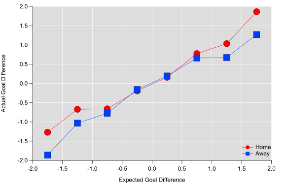
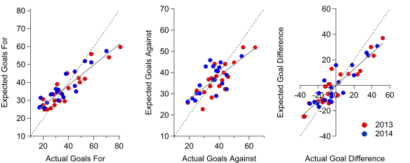
Below are some plots and a summary table comparing actual goals to expected goals for each team in the dataset. The correlation is stronger for goals for than against, although the bias is larger also as the ‘best’ teams tend to score more than expected and the ‘worst’ teams score fewer than expected. Looking at goal difference, the relationship is very strong over a season.
I also performed several out-of-sample tests to test the regressions by spitting the data-set into two sets (2012/13-2013/14 and 2014/15 only) and ran cross-validation tests on them. The model performed well out-of-sample, with the summary statistics being broadly similar when compared to the in-sample tests.

Comparison between actual goals and expected goals. Red dots are individual teams in each season. Dashed black line is 1:1 line and solid black line is the line of best fit.

Comparison between actual goals and expected goals. MAE refers to Mean Absolute Error, while slope and intercept are calculated from a linear regression between the actual and expected totals.
I also ran the regression on possessions ending in shots and the results were broadly quite similar, although I would say that the shot-based expected goal model performed slightly better overall. Overall, the non-shots based expected goals model is very good at explaining past performance and is comparable to more traditional expected goal models.
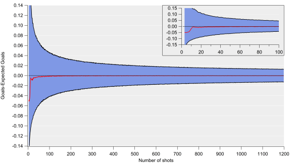
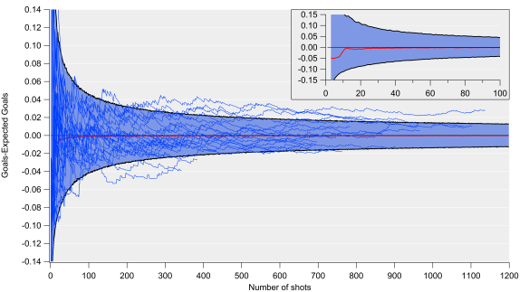
On the predictive side, I ran a similar test to what Michael Caley did here as a quick check of how well the model did. I looked at each clubs matches in chronological order and calculated how well the expected goal models predicted actual goals in their next 19 matches (half a season in the Premier League) using an increasing number of prior matches to base the prediction on. For example, for a 10 match sample, I started at matches 1-10 and calculated statistics for matches 11-30, followed by matches 2-11 for matches 12-31 and so on.
Note that the ‘wiggles’ in the data are due to the number of teams changing as we move from one seasons worth of games to another i.e. some teams have only 38 games worth of matches, while others have 114. I also ran the same analysis for the next 38 matches and found similar features to those outlined below. I also did out-of-sample validation tests and found similar results, so I’m just showing the full in-sample tests below.

Capability of non-shot based and shot-based expected goals to predict future goals over the next 19 matches using differing numbers of previous matches as the input. Actual goals are also shown for reference. R-squared is shown on the left, while the mean absolute error is shown on the right.
I’m not massively keen on using r-squared as a diagnostic for predictions, so I also calculated the mean absolute errors for the predictions. The non-shots expected goals model performs very well here and compares very favourably with the shots-based version (the errors and correlations are typically marginally better). After around 20-30 matches, expected goals and actual goals converge in terms of their predictive capability – based on some other diagnostic tests I’ve run, this is around the point where expected goals tends to ‘match’ quite well with actual goals i.e. actual goals regresses to our mean expectation, so this convergence here is not too surprising.
The upshot is that the expected goal models perform very well and are a better predictor of future goals than goals themselves, particularly over small samples. Furthermore, they pick up information about future performance very quickly as the predictive capability tends to flat-line after less than 10 matches. I plan to expand the model to include set-play possessions and perform point projections, where I will do some more extensive investigation of the predictive performance of the model but I would say this is an encouraging start.
Bonus round
Below are the current expected goal difference rankings for the current Premier League season. The numbers are based on the regression I performed on the 2012/13-2014/15 dataset. I’ll start posting more figures as the season continues on my Twitter feed.
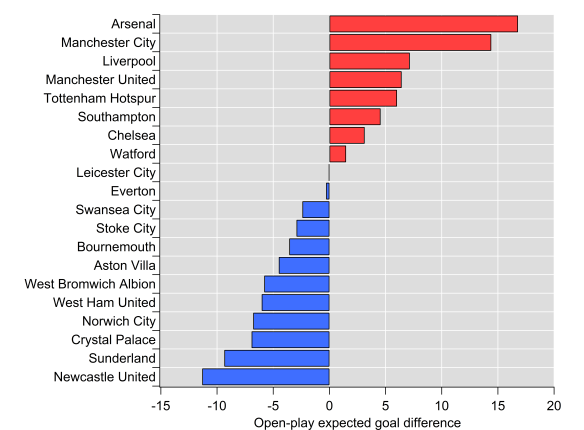
Open-play expected goal difference totals after 19 games of the 2015/16 Premier League season.