More thinking about goalkeepers

Following my previous article on the shot-stopping ability of goalkeepers, Mike Goodman posed an interesting question on Twitter:

This is certainly not an annoying question and I tend to think that such questions should be encouraged in the analytics community. Greater discussion should stimulate further work and enrich the community.

It certainly stands to reason and observation that goalkeepers can influence a strikers options and decision-making when shooting but extracting robust signals of such a skill may prove problematic.

To try and answer this question, I built a quick model to calculate the likelihood that a non-blocked shot would end up on target. It’s essentially the same model as in my previous post but for expected shots on target rather than goals. The idea behind the model is that goalkeepers who are able to ‘force’ shots off-target would have a net positive rating when subtracting actual shots on target from the expected rate.

When I looked at the results, two of the standout names were Gianluigi Buffon and Jan Oblak; Buffon is a legend of the game and up there with the best of all time, while Oblak is certainly well regarded, so not a bad start.

However, after delving a little deeper, dragons started appearing in the analysis.

In theory, goalkeepers influencing shot-on-target rates would do so for shots closer to goal as they would narrow the amount of goal they can aim for via their positioning. However, I found the exact opposite. Further investigation of the model workings pointed to the problem – the model showed significant biases depending on whether the shot was inside or outside the area.

This is shown below where actual and expected shot-on-target totals for each goalkeeper are compared. For shots inside the box, the model tends to under-predict, while the opposite is the case for outside the box shots. These two biases cancelled each other out when looking at the full aggregated numbers (the slope was 0.998 for total shots-on-target vs the expected rate).

Act_vs_Ex_SoT.png

Actual vs expected shots-on-target totals for goalkeepers considered in the analysis. Dashed line is the 1:1 line, while the solid line is the line of best fit. Left-hand plot is for shots inside the box, while the right-hand plot is for shots outside the box. Data via Opta.

The upshot of this was that goalkeepers performing well-above expectation were doing so due to shots from longer-range being off-target when compared to the expected rates for the model. I suspect that the lack of information on defensive pressure is skewing the results and introducing bias into the model.

Now when we think of Buffon and Oblak performing well, we recall that they play behind probably the two best defenses in Europe at Juventus and Atlético respectively. Rather than ascribing the over-performance to goalkeeping skill, the effect is likely driven by the defensive pressure applied by their team-mates and issues with the model.

Exploring model performance is something I’ve written about previously and I would also highly recommend this recent article by Garry Gelade on assessing expected goals. While the above is an unsatisfactory ending for the analysis, it does illustrate the importance of testing model output prior to presenting results and testing whether such results match with our theoretical expectations.

Knowing what questions analytics can and cannot answer is a pretty useful thing to know. Better luck next time hopefully.


Advertisement

Uncertain expectations

In this previous post, I describe a relatively simple version of an expected goals model that I’ve been developing recently. In this post, I want to examine the limitations and uncertainties relating to how well the model predicts goals.

Just to recap, I built the model using data from the Premier League from 2013/14 and 2014/15. For the analysis below, I’m just going to focus on non-penalty shots with the foot, so it includes both open-play and set piece shot situations. Mixing these will introduce some bias but we have to start somewhere. The data amounts to over 16,000 shots.

What follows is a long and technical post. You have been warned.

Putting the boot in

One thing to be aware of is how the model might differ if we used a different set of shots for input; ideally the answer we get shouldn’t change if we only used a subset of the data or if we resample the data. If the answer doesn’t change appreciably, then we can have more confidence that the results are robust.

Below, I’ve used a statistical technique known as ‘bootstrapping‘ to assess how robust the regression is for expected goals. Bootstrapping belongs to a class of statistical methods known as resampling. The method works by randomly extracting shots from the dataset and rerunning the regression many times (1000 times in the plot below). Using this, I can estimate a confidence interval for my expected goal model, which should provide a reasonable estimate of goal expectation for a given shot.

For example, the base model suggests that a shot from the penalty spot has an xG value of 0.19. The bootstrapping suggests that the 90% confidence interval gives an xG range from 0.17 to 0.22. What this means is that on 90% of occasions that Premier League footballers take a shot from the penalty spot, we would expect them to score somewhere between 17-22% of the time.

The plot below shows the goal expectation for a shot taken in the centre of the pitch at varying distances from the goal. Generally speaking, the confidence interval range is around ±1-2%. I also ran the regressions on subsets of the data and found that after around 5000 shots, the central estimate stabilised and the addition of further shots in the regression just narrows the confidence intervals. After about 10,000 shots, the results don’t change too much.

Test.

Expected goal curve for shots in the centre of the pitch at varying distances from the goal. Shots with the foot only. The red line is the median expectation, while the blue shaded region denotes the 90% confidence interval.

I can use the above information to construct a confidence interval for the expected goal totals for each team, which is what I have done below. Each point represents a team in each season and I’ve compared their expected goals vs their actual goals. The error bars show the range for the 90% confidence intervals.

Most teams line up with the one-to-one line within their respective confidence intervals when comparing with goals for and against. As I noted in the previous post, the overall tendency is for actual goals to exceed expected goals at the team level.

Expected goals vs actual goals for teams in the 2013/14 and 2014/15 Premier League. Dotted line is the 1:1 line, the solid line is the line of best fit and the error bars denote the 90% confidence intervals based on the xG curve above.

Expected goals vs actual goals for teams in the 2013/14 and 2014/15 Premier League. Dotted line is the 1:1 line, the solid line is the line of best fit and the error bars denote the 90% confidence intervals based on the xG curve above.

As an example of what the confidence intervals represent, in the 2013/14 season, Manchester City’s expected goal total was 59.8, with a confidence interval ranging from 52.2 to 67.7 expected goals. In reality, they scored 81 non-penalty goals with their feet, which falls outside of their confidence interval here. On the plot below, Manchester City are the red marker on the far right of the expected goals for vs actual goals for plot.

Embracing uncertainty

Another method of testing the model is to look at the model residuals, which are calculated by subtracting the outcome of a shot (either zero or one) from its expected goal value. If you were an omnipotent being who knew every aspect relating to the taking of a shot, you could theoretically predict the outcome of a shot (goal or no goal) perfectly (plus some allowance for random variation). The residuals of such a model would always be zero as the outcome minus the expectation of a goal would equal zero in all cases. In the real world though, we can’t know everything so this isn’t the case. However, we might expect that over a sufficiently large sample, the residual will be close to zero.

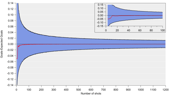
In the figure below, I’ve again bootstrapped the data and looked at the model residuals as the number of shots increases. I’ve done this 10,000 times for each number of shots i.e. I extract a random sample from the data and then calculate the residual for that number of shots. The red line is the median residual (goals minus expected goals), while the blue shaded region corresponds to the standard error range (calculated as the 90% confidence interval). The residual is normalised to a per shot basis, so the overall uncertainty value is equal to this value multiplied by the number of shots taken.
BootStrap_xGdiff_col

Goals-Expected Goals versus number of shots calculated via bootstrapping. Inset focusses on the first 100 shots. The red line is the median, while the blue shaded region denotes the 90% confidence interval (standard error).

The inset shows how this evolves up to 100 shots and we see that over about 10 shots, the residual approaches zero but the standard errors are very large at this point. Consequently, our best estimate of expected goals is likely highly uncertain over such a small sample. For example, if we expected to score two goals from 20 shots, the standard error range would span 0.35 to 4.2 goals. To add a further complication, the residuals aren’t normally distributed at that point, which makes interpretations even more challenging.

Clearly there is both a significant amount of variation over such small samples, which could be a consequence of both random variation and factors not included in the model. This is an important point when assessing xG estimates for single matches; while the central estimate will likely have a very small residual, the uncertainty range is huge.

As the sample size increases, the uncertainty decreases. After 100 shots, which would equate to a high shot volume for a forward, the uncertainty in goal expectation would amount to approximately ±4 goals. After 400 shots, which is close to the average number of shots a team would take over a single season, the uncertainty would equate to approximately ±9 goals. For a 10% conversion rate, our expected goal value after 100 shots would be 10±4, while after 400 shots, our estimate would be 40±9 (note the percentage uncertainty decreases as the number of shots increases).
BootStrap_xGdiff_col_wTeams

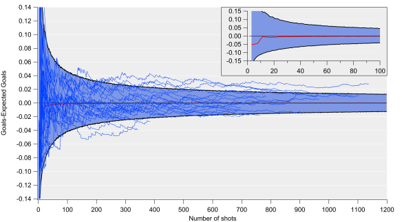
Same as above but with individual teams overlaid.

Above is the same plot but with the residuals shown for each team over the past two seasons (or one season if they only played for a single season). The majority of teams fall within the uncertainty envelope but there are some notable deviations. At the bottom of the plot are Burnley and Norwich, who significantly under-performed their expected goal estimate (they were also both relegated). On the flip side, Manchester City have seemingly consistently outperformed the expected goal estimate. Part of this is a result of the simplicity of the model; if I include additional factors such as how the chance is created, the residuals are smaller.

How well does an xG model predict goals?

Broadly speaking, the central estimates of expected goals appear to be reasonably good; the residuals tend to zero quickly and even though there is some bias, the correlations and errors are encouraging. When the uncertainties in the model are propagated through to the team level, the confidence intervals are on average around ±15% for expected goals for and against.

When we examine the model errors in more detail, they tend to be larger (around ±25% at the team level over a single season). The upshot of all this is that there appears to be a large degree of uncertainty in expected goal values when considering sample sizes relevant at the team and player level. While the simplicity of the model used here may mean that the uncertainty values shown represent a worst-case scenario, it is still something that should be considered when analysts make statements and projections. Having said this, based on some initial tests, adding extra complexity doesn’t appear to reduce the residuals to any great degree.

Uncertainty estimates and confidence intervals aren’t sexy and having spent the last 1500ish words writing about them, I’m well aware they aren’t that accessible either. However, I do think they are useful and important in the real world.

Quantifying these uncertainties can help to provide more honest assessments and recommendations. For example, I would say it is more useful to say that my projections estimate that player X will score 0.6-1.4 goals per 90 minutes next season along with some central value, rather than going with a single value of 1 goal per 90 minutes. Furthermore, it is better to state such caveats in advance – if you just provided the central estimate and the player posted say 0.65 goals per 90 and you then bring up your model’s uncertainty range, you will just sound like you’re making excuses.

This also has implications regarding over and under performance by players and teams relative to expected goals. I frequently see statements about regression to the mean without considering model errors. As George Box wisely noted:

Statisticians, like artists, have the bad habit of falling in love with their models.

This isn’t to say that expected goal models aren’t useful, just that if you want to wade into the world of probability and modelling, you should also illustrate the limitations and uncertainties associated with the analysis.

Perhaps those using expected goal models are well aware of these issues but I don’t see much discussion of it in public. Analytics is increasingly finding a wider public audience, along with being used within clubs. That will often mean that those consuming the results will not be aware of these uncertainties unless you explain them. Speaking as a researcher who is interested in the communication of science, I can give many examples of where not discussing uncertainty upfront can backfire in the long run.

Isn’t uncertainty fun!

——————————————————————————————————————–

Thanks to several people who were kind enough to read an initial draft of this article and the proceeding method piece.

Stats! What are they good for?

I’ve been closely following the developments in the football analytics community for close to two years now, ever since WhoScored allied themselves with the Daily Mail and suggested Xavi wasn’t so good at the football and I was directed to James Grayson’s wonderful riposte.

There has been some discussion on Twitter about the state of football analytics recently and I thought I would commit some extended thoughts on this topic to writing.

Has football analytics stalled?

Part of the Soccermetrics podcast, featuring Howard Hamilton and Zach Slaton, revolved around how football analytics as an activity has “stalled” (Howard has since attributed the “stalled” statement to Chris Anderson, although he seemingly agrees with it). Even though this wasn’t really defined, I find it difficult to comprehend the view that analytics has stalled.

Over the past two years, the community has developed a lot as far as I can see. James Grayson and Mark Taylor continue to regularly publish smart work, while new bloggers have emerged also. The StatsBomb website has brought together a great collection of analysts and thinkers on the game and they appear to be gaining traction outside of the analytics echo chamber.

In addition to this, data is increasingly finding a place in the mainstream media; Zach Slaton writes at Forbes, Sean Ingle is regularly putting numbers into his Guardian columns and there is a collection of writers contributing to the Dutch newspaper De Volkskrant. Mike Goodman is doing some fantastic work at Grantland; his piece on Manchester United this season is an all too rare example of genuine insight in the wider football media. The Numbers Game book by Chris Anderson and David Sally was also very well received.

Allied to these writing developments, a number of analytics bloggers have joined professional clubs or data organisations recently – surely it is encouraging to see smart people being brought into these environments? (One side effect of this is that some great work is lost from the public sphere though e.g. the StatDNA blog).

To me, this all seems like progress on a number of fronts.

What are we trying to achieve?

The thing that isn’t clear to me is what people in the analytics community are actually aiming for. Some are showcasing their work with the aim of getting a job in the football industry, some are hoping to make some money, while others are doing it as a hobby (*waves hand*). Whatever the motivation, the work coming out of the community is providing insights, context and discussion points and there is an audience for it even if it is considered quite niche.

Football analytics is still in its infancy and expecting widespread acceptance in the wider football community at this stage is perhaps overly ambitious. However, strides are being made; tv coverage has started looking more at shot counts over a season and heat maps of touches have made a few appearances. These are small steps undoubtedly but I doubt there is much demand for scatter plots, linear regression and statistical significance tests from tv producers. Simple and accessible tables or metrics that can be overlaid on an image of a football pitch seem to go down well with a broader audience – the great work being done on shot locations seems ripe for this as it is accessible and intuitive without resorting to complex statistical language.

Gary Neville shows off his massive iPad.

Gary Neville shows off his massive iPad. Courtesy of thedrum.com.

However, I don’t think the media should be the be all and end all for judging the success or progress of football analytics. Fan discussion of football is increasingly found online in the form of blogs, forums and Twitter, so the media don’t have to be the gatekeepers to analytics content. Saying that, I would love to see more intelligent discussion of football in the media and I feel that analytics is well placed to contribute to that. I’d be interested to hear what it is people in the football analytics community are aiming for in the longer term.

What about the clubs?

The obvious aspect of the analytics community that I’ve omitted from the discussion so far is the role of the clubs in all this. It’s difficult to know what goes on within clubs due to their secrecy. The general impression I get is that there are analytics teams toiling away but without necessarily making an impact in decision making at the club, whether that is in terms of team analysis or in the transfer market. Manchester City are one example of a team using data for such things based on this article.

With this in mind, I was interested to listen to the Sky Sports panel discussion show featuring Chris Anderson, Damien Commoli and Sam Allardyce. Chris co-authored the excellent The Numbers Game book and brought some nuance and genuine insight to the discussion. Commoli is mates with Billy Beane. Allardyce is held up as an acolyte for football analytics at the managerial level in English football and I think this is first time I’ve really heard him speak about it. I wasn’t impressed.

Allardyce clearly takes an interest in the numbers side of the game and reeled off plenty of figures, which on the surface seemed impressive. He seemingly revels in the idea that he is some sort of visionary with his interest in analytics, repeating on several occasions how he has been using data for over ten years. He seemed particularly pleased with the “discovery” of how many clean sheets, goals and other aspects of the game were required to gain a certain number of points in the Premier League; something that many analysts could work out in their lunch hour given the appropriate data.

I would question how this analysis and many of the other nuggets he threw out are actually actionable though; much of this is just stamp-collecting and doesn’t really move things forward in terms of actually identifying what is happening at the process level on the pitch. For example, Commoli’s statistic on a team never losing when having ten or more shots on goal, which is valuable information for those footballers who don’t aim for the goal. Now it could be that they were holding back the good stuff but several of their comments suggested they don’t really understand core analytics concepts such as regression to the mean and the importance of sample size e.g. referring to Aaron Ramsey’s unsustainable early-season scoring run. I would have expected more from people purporting to be leading take up of analytics at club level.

I felt Allardyce’s comment about his “experience” being better than “maths” when discussing the relationship between money and success betrayed his actual regard for the numbers side of football. Many of the numbers he quoted seemed to be used to confirm his own ideas about the game. This is fine but I think to genuinely gain an edge using analytics, you need to see where the data takes you and make it actionable. This is hard and is something that the analytics community could do better (Paul Riley is doing great work on his blog in this area for goalkeepers). The context that analytics provides is very valuable but without identifying “why” certain patterns are observed, it is difficult to alter the process on the field.

Based on the points that Allardyce made, I have my doubts whether the clubs are any further ahead in this regard than what is done publicly by the online analytics community. If there is a place where analytics has stagnated, maybe it is the within the clubs. To my mind, they would do well to look at what is going on in the wider community and try to tap into that more.

——————————————————————————————————————–

Shorter version of this post, courtesy of Edward Monkton.

Where are we Going?

I don’t know, I thought you knew.

No I don’t know. Maybe he knows.

No, He definitely doesn’t know.

*PAUSE*

Maybe no-one knows.

*PAUSE*

Oh Well. I hope it’s nice when we get there.