More thinking about goalkeepers

Following my previous article on the shot-stopping ability of goalkeepers, Mike Goodman posed an interesting question on Twitter:

This is certainly not an annoying question and I tend to think that such questions should be encouraged in the analytics community. Greater discussion should stimulate further work and enrich the community.

It certainly stands to reason and observation that goalkeepers can influence a strikers options and decision-making when shooting but extracting robust signals of such a skill may prove problematic.

To try and answer this question, I built a quick model to calculate the likelihood that a non-blocked shot would end up on target. It’s essentially the same model as in my previous post but for expected shots on target rather than goals. The idea behind the model is that goalkeepers who are able to ‘force’ shots off-target would have a net positive rating when subtracting actual shots on target from the expected rate.

When I looked at the results, two of the standout names were Gianluigi Buffon and Jan Oblak; Buffon is a legend of the game and up there with the best of all time, while Oblak is certainly well regarded, so not a bad start.

However, after delving a little deeper, dragons started appearing in the analysis.

In theory, goalkeepers influencing shot-on-target rates would do so for shots closer to goal as they would narrow the amount of goal they can aim for via their positioning. However, I found the exact opposite. Further investigation of the model workings pointed to the problem – the model showed significant biases depending on whether the shot was inside or outside the area.

This is shown below where actual and expected shot-on-target totals for each goalkeeper are compared. For shots inside the box, the model tends to under-predict, while the opposite is the case for outside the box shots. These two biases cancelled each other out when looking at the full aggregated numbers (the slope was 0.998 for total shots-on-target vs the expected rate).

Act_vs_Ex_SoT.png

Actual vs expected shots-on-target totals for goalkeepers considered in the analysis. Dashed line is the 1:1 line, while the solid line is the line of best fit. Left-hand plot is for shots inside the box, while the right-hand plot is for shots outside the box. Data via Opta.

The upshot of this was that goalkeepers performing well-above expectation were doing so due to shots from longer-range being off-target when compared to the expected rates for the model. I suspect that the lack of information on defensive pressure is skewing the results and introducing bias into the model.

Now when we think of Buffon and Oblak performing well, we recall that they play behind probably the two best defenses in Europe at Juventus and Atlético respectively. Rather than ascribing the over-performance to goalkeeping skill, the effect is likely driven by the defensive pressure applied by their team-mates and issues with the model.

Exploring model performance is something I’ve written about previously and I would also highly recommend this recent article by Garry Gelade on assessing expected goals. While the above is an unsatisfactory ending for the analysis, it does illustrate the importance of testing model output prior to presenting results and testing whether such results match with our theoretical expectations.

Knowing what questions analytics can and cannot answer is a pretty useful thing to know. Better luck next time hopefully.


Advertisement

Thinking about goalkeepers

Goalkeepers have typically been a tough nut to crack from a data analytics point-of-view. Randomness is an inherent aspect of goal-scoring, particularly over small samples, which makes drawing robust conclusions at best challenging and at worst foolhardy. Are we identifying skill in our ratings or are we just being sent down the proverbial garden path by variance?

To investigate some of these issues, I’ve built an expected save model that takes into account shot location and angle, whether the shot is a header or not and shot placement. So a shot taken centrally in the penalty area sailing into the top-corner will be unlikely to be saved, while a long-range shot straight at the keeper in the centre of goal should usually prove easier to handle.

The model is built using data from the past four seasons of the English, Spanish, German and Italian top leagues. Penalties are excluded from the analysis.

Similar models have been created by new Roma analytics guru, Stephen McCarthy, Colin Trainor & Constantinos Chappas and Thom Lawrence in the past.

The model thus provides an expected goal value for each shot that a goalkeeper faces, which we can then compare with the actual outcome. In a simpler world, we could easily identify shot-stopping skill by taking the difference between reality and expectation and then ranking goalkeepers by who has the best (or worst) difference.

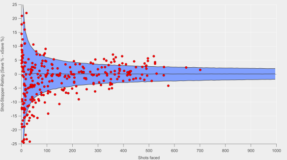
However, this isn’t a simple world, so we run into problems like those illustrated in the graphic below.

Keeper_Funnel_Plot.png

Shot-stopper-rating (actual save percentage minus expected save percentage) versus number of shots faced. The central black line at approximately zero is the median, while the blue shaded region denotes the 90% confidence interval. Red markers are individual players. Data via Opta.

Each individual red marker is a player’s shot-stopper rating over the past four seasons versus the number of shots they’ve faced. We see that for low shot totals, there is a huge range in the shot-stopper-ranking but that the spread decreases as the number of shots increases, which is an example of regression to the mean.

To illustrate this further, I used a technique called boot-strapping to re-sample the data and generate confidence intervals for an average goalkeeper. This re-sampling is done 10,000 times to create a probability distribution built by randomly extracting groups of shots from the data-set and calculating actual and expected save percentages and then seeing how large the difference is. We see a strong narrowing of the blue uncertainty envelope up to around 50 shots, with further narrowing up to about 200 shots. After this, the narrowing is less steep.

What this effectively means is that there is a large band of possible outcomes that we can’t realistically separate from noise for an average goalkeeper. Over a season, a goalkeeper faces a little over 100 shots on target (119 on average according to the data used here). Thus, there is a huge opportunity for randomness to play a role and it is therefore of little surprise to find that there is little repeatability year-on-year for save percentage.

Things do start to settle down as shot totals increase though. After 200 shots, a goalkeeper would need to be performing more than ± 4% on the shot-stopper-rating scale to stand up to a reasonable level of statistical significance. After 400 shots, signal is easier to discern with a keeper needing to register more than ± 2% to emerge from the noise. That is not to say that we should be beholden to statistical significance but it is certainly worth bearing in mind in any assessment plus an understanding of the uncertainty inherent in analytics can be a powerful weapon to wield.

What we do see in the graphic above are many goalkeepers outside of the blue uncertainty envelope. This suggests that we might be able to identify keepers who are performing better or worse than the average goalkeeper, which would be pretty handy for player assessment purposes. Luckily, we can employ some more maths courtesy of Pete Owen who presented a binomial method to rank shot-stopping performance in a series of posts available here and here.

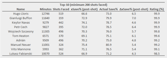
The table below lists the top-10 goalkeepers who have faced more than 200 shots over the past four seasons by the binomial ranking method.

GK-Top10.png

Top-10 goalkeepers as ranked by their binomial shot-stopper-ranking. Post-shot refers to expected save model that accounts for shot placement. Data via Opta.

I don’t know about you but that doesn’t look like too shabby a list of the top keepers. It may be that some of the names on the list have serious flaws in their game aside from shot-stopping but that will have to wait another day and another analysis.

So where does that leave us in terms of goalkeeping analytics? On one hand, we have noisy unrepeatable metrics from season-to-season. On the other, we appear to have some methods available to extract the signal from the noise over larger samples. Even then, we might be being fooled by aspects not included in the model or the simple fact that we expect to observe outliers.

Deficiencies in the model are likely our primary concern but these should be checked by a skilled eye and video clips, which should already be part of the review process (quit sniggering at the back there). Consequently, the risks ingrained in using an imperfect model can be at least partially mitigated against.

Requiring 2-3 seasons of data to get a truly robust view on shot-stopping ability may be too long in some cases. However, perhaps we can afford to take a longer-term view for such an important position that doesn’t typically see too much turnover of personnel compared to other positions. The level of confidence you might want when short-listing might well depend on the situation at hand; perhaps an 80% chance of your target being an above average shot-stopper would be palatable in some cases?

All this is to say that I think you can assess goalkeepers by the saves they do or do not make. You just need to be willing to embrace a little uncertainty in the process.

Identifying and assessing team-level strategies: 2017 OptaPro Forum Presentation

At the recent OptaPro Analytics Forum, I was honoured to be selected to present for a second time to an audience of analysts and other representatives from the sporting industry. My aim was to explore the multifaceted approaches employed by teams using cluster analysis of possession chains.

My thinking was that this could be used to assess the strengths and weaknesses of teams in both attack and defense, which could be used for opposition scouting. The results can also be used to evaluate how well players contribute to certain styles of play and potentially use this in recruitment.

The video of the presentation is below, so go ahead and watch it for more details. The slides are available here and I’ve pulled out some of the key graphics below.

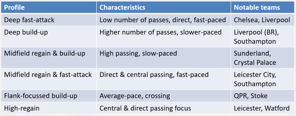
The main types of attacking moves that result in shots are in the table below. I used the past four full English Premier League seasons plus the current 2016/17 season for the analysis here but an obvious next step is to expand the analysis across multiple leagues.

Cluster Profile Summary.png

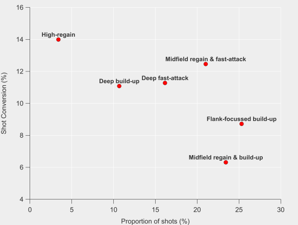
Below is a comparison of the efficiency (in terms of shot conversion) and frequency of these attack types. The value of regaining the ball closer to goal and quickly transitioning into attack is clear, while slower or flank-focussed build-up is less potent. Much of the explanation for these differences in conversion rate can be linked to the distance from which such shots are taken on average.

An interesting wrinkle is the similarity in conversion rates between the ‘deep build-up’ and ‘deep fast-attacks’ profiles, with shots taken in the build-up focussed profile being approximately 2 yards further away from goal on average than the faster attacks. Looking through examples of the ‘deep build-up’ attacks, these are often characterised by periods of ball circulation in deeper areas followed by a quick transition through the opposition half towards goal with the opposition defense caught higher up the pitch, which may explain the results somewhat.

EfficiencyVsFrequency

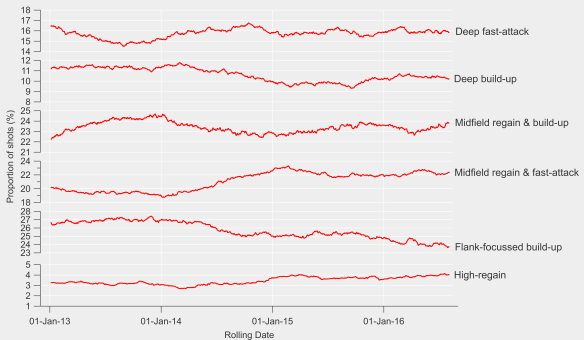
Finally, here is a look at how attacking styles have evolved over time. The major changes are the decline in ‘flank-focussed build-up’ and increase in the ‘midfield regain & fast attack’ profile, which is perhaps unsurprising given wider tactical trends and the managerial changes over the period. There is also a trend in attacks from deep being generated from faster-attacks rather than build-up focussed play. A greater emphasis on transitions coupled with fast/direct attacking appears to have emerged across the Premier League.

EPL_ProfileTimeline

These are just a few observations and highlights from the presentation and I’ll hopefully put together some more team and player focussed work in the near future. It has been nearly a year since my last post but hopefully I’ll be putting out a steadier stream of content over the coming months.

Fools Gold: xG +/-

Football is a complex game that has many facets that are tough to represent with numbers. As far as public analytics goes, the metrics available are best at assessing team strength, while individual player assessments are strongest for attacking players due to their heavy reliance on counting statistics relating to on-the-ball numbers. This makes assessing defenders and goalkeepers a particular challenge as we miss the off-ball positional adjustments and awareness that marks out the best proponents of the defensive side of the game.

One potential avenue is to examine metrics from a ‘top-down’ perspective i.e. we look at overall results and attempt to untangle how a player contributed to that result. This has the benefit of not relying on the incomplete picture provided by on-ball statistics but we do lose process level information on how a player contributes to overall team performance (although we could use other methods to investigate this).

As far as football is concerned, there are a few methods that aim to do this, with Goalimpact being probably the most well-known. Goalimpact attempts to measure ‘the extent that a player contributes to the goal difference per minute of a team’ via a complex method and impressively broad dataset. Daniel Altman has a metric based on ‘Shapley‘ values that looks at how individual players contribute to the expected goals created and conceded while playing.

Outside of football, one of the most popular statistics to measure player contribution to overall results is the concept of plus-minus (or +/-) statistics, which is commonly used within basketball, as well as ice hockey. The most basic of these metrics simply counts the goals or points scored and conceded while a player is on the pitch and comes up with an overall number to represent their contribution. There are many issues with such an approach, such as who a player is playing along side, their opponent and the venue of a match; James Grayson memorably illustrated some of these issues within football when WhoScored claimed that Barcelona were a better team without Xavi Hernández.

Several methods exist in other sports to control for these factors (basically they add in a lot more maths) and some of these have found their way to football. Ford Bohrmann and Howard Hamilton had a crack at the problem here and here respectively but found the results unsatisfactory. Martin Eastwood used a Bayesian approach to rate players based on the goal difference of their team while they are playing, which came up with more encouraging results.

Expected goals

One of the potential issues with applying plus-minus to football is the low scoring nature of the sport. A heavily influential player could play a run of games where his side can’t hit the proverbial barn door, whereas another player could be fortunate to play during a hot-streak from one of his fellow players. Goal-scoring is noisy in football, so perhaps we can utilise a measure that irons out some of this noise but still represents a good measure of team performance. Step forward expected goals.

Instead of basing the plus-minus calculation on goals, I’ve used my non-shot expected goal numbers as the input. The method splits each match into separate periods and logs which players are on the pitch at a given time. A new segment starts when a lineup changes i.e. when a substitution occurs or a player is sent off. The expected goals for each team are then calculated for each period and converted to a value per 90 minutes. Each player is a ‘variable’ in the equation, with the idea being that their contribution to a teams expected goal difference can be ‘solved’ via the regression equation.

For more details on the maths side of plus-minus, I would recommend checking out Howard Hamilton’s article. I used ridge regression, which is similar to linear regression but the calculated coefficients tend to be pulled towards zero (essentially it increases bias while limiting huge outliers, so there is a tradeoff between bias and variance).

As a first step, I’ve calculated the plus-minus figures over the previous three English Premier League seasons (2012/13 to 2014/15). Every player that has appeared in the league is included as I didn’t find there was much difference when excluding players under a certain threshold of minutes played (this also avoids having to include such players in some other manner, which is typically done in basketball plus-minus). However, estimates for players with fewer than approximately 900 minutes played are less robust.

The chart below shows the proportion of players with a certain plus-minus score per 90 minutes played. As far as interpretation goes, if we took a team made up of 11 players, each with a plus-minus score of zero, the expected goal difference of the team would add up to zero. If we then replaced one of the players with one with a plus-minus of 0.10, the team’s expected goal difference would be raised to 0.10.

PM_Dist.png

Distribution of xG plus-minus scores.

The range of plus-minus scores is from -0.15 to 0.15, so replacing a player with a plus-minus score of zero with one with a score of 0.15 would equate to an extra 5.7 goals over a Premier League season. Based on this analysis by James Grayson, that would equate to approximately 3.5-4.0 points over a season on average. This is comparable to figures published relating to calculations based on the Goalimpact metric system discussed earlier. That probably seems a little on the low side for what we might generally assume would be the impact of a single player, which could point towards the method either narrowing the distribution too much (my hunch) or an overestimate in our intuition. Validation will have to wait for another day

Most valuable players

Below is a table of the top 13 players according to the model. Vincent Kompany is ranked the highest by this method; on one hand this is surprising given the often strong criticism that he receives but then on the other, when he is missing, those replacing him in Manchester City’s back-line look far worse and the team overall suffers. According to my non-shots xG model, Manchester City have been comfortably the best team over the previous three seasons and are somewhat accordingly well-represented here.

xG_PM_Top10_Table

Top 13 players by xG plus-minus scores for the 2012/13-2014/15 Premier League seasons. Minimum minutes played was 3420 i.e. equivalent to a full 38 match season.

Probably the most surprising name on the list is at number three…step forward Joe Allen! I doubt even Joe’s closest relatives would rate him as the third best player in the league but I think that what the model is trying to say here is that Allen is a very valuable cog who improves the overall performance level of the team. Framed in that way, it is perhaps slightly more believable (if only slightly) that his skill set gets more out of his team mates. When fit, Allen does bring added intelligence to the team and as a Liverpool fan, ‘intelligence’ isn’t usually a word I associate with the side. Highlighting players who don’t typically stand-out is one of the goals of this sort of analysis, so I’ll run with it for now while maintaining a healthy dose of skepticism.

I chose 13 as the cutoff in the table so that the top goalkeeper on the list, Hugo Lloris, is included so that an actual team could be put together. Note that this doesn’t factor in shot-stopping (I’ve actually excluded rebound shots, which might have been one way for goalkeepers to influence the scores more directly), so the rating for goalkeepers should be primarily related to other aspects of goalkeeping skills. Goalkeepers are probably still quite difficult to nail down with this method due to them rarely missing matches though, so there is a fairly large caveat with their ratings.

Being as this is just an initial look, I’m going to hold off on putting out a full list but I definitely will do in time once I’ve done some more validation work and ironed out some kinks.

Validation, Repeatability & Errors

Fairly technical section. You’ve been warned.

One of the key facets of using ridge regression is choosing a ‘suitable’ regularization parameter, which is what controls the bias-to-variance tradeoff; essentially larger values will pull the scores closer to zero. Choosing this objectively is difficult and in reality, some level of subjectivity is going to be involved at some stage of the analysis. I did A LOT of cross-validation analysis where I split the match segments into even and odd sets and ran the regression while varying a bunch of parameters (e.g. minutes cutoff, weighting of segment length, the regularization value). I then looked at the error between the regression coefficients (the player plus-minus scores) in the out-of-sample set compared to the in-sample set to choose my parameters. For the regularization parameter, I chose a value of 50 as that was where the error reached a minimum initially with relatively little change for larger values.

I also did some repeatability testing comparing consecutive seasons. As is common with plus-minus, the repeatability is very limited. That isn’t much of a surprise as the method is data-hungry and a single season doesn’t really cut it for most players. The bias introduced by the regularization doesn’t help either here. I don’t think that this is a death-knell for the method though, given the challenges involved and the limitations of the data.

In the table above, you probably noticed I included a column for errors, specifically the standard error. Typically, this has been where plus-minus has fallen down, particularly in relation to football. Simply put, the errors have been massive and have rendered interpretation practically impossible e.g. the errors for even the most highly rated players have been so large that statistically speaking it has been difficult to evaluate whether a player is even ‘above-average’.

I calculated the errors from the ridge regression via bootstrap resampling. There are some issues with combining ridge regression and bootstrapping (see discussion here and page 18 here) but these errors should give us some handle on the variability in the ratings.

You can see above that the errors are reasonably large, so the separation between players isn’t as good as you would want. In terms of their magnitude relative to the average scores, the errors are comparable to those I’ve found published for basketball. That provides some level of confidence as they’ve been demonstrated to have genuine utility there. Note that I’ve not cherry-picked the players above in terms of their standard errors either; encouragingly the errors don’t show any relationship with minutes played after approximately 900 minutes.

The gold road’s sure a long road

That is essentially it so far in terms of what I’m ready to share publicly. In terms of next steps, I want to expand this to include other leagues so that the model can keep track of players transferring in and out of a league. For example, Luis Suárez disappears when the model reaches the 2014/15 season, when in reality he was settling in quite nicely at Barcelona. That likely means that his rating isn’t a true reflection of his overall level over the period.

Evaluating performance over time is also a big thing I want to be able to do; a three year average is probably not ideal, so either some weighting for more recent seasons or a moving two season window would be better. This is typically what has been done in basketball and based on initial testing, it doesn’t appear to add more noise to the results.

Validating the ratings in some fashion is going to be a challenge but I have some ideas on how to go about that. One of the advantages of plus-minus style metrics is that they break-down team level performance to the player level, which is great as it means that adding the players back up into a team or squad essentially correlates perfectly with team performance (as represented by expected goals here). However, that does result in a tautology if the validation is based on evaluating team performance unless there are fundamental shifts in team makeup e.g. a large number of transfers in and out of a squad or injuries to key personnel.

This is just a start, so there will be more to come over time. The aim isn’t to provide a perfect representation of player contribution but to add an extra viewpoint to squad and player evaluation. Combining it with other data analysis and scouting would be the longer-term goal.

I’ll leave you with piano carrier extradionaire, Joe Allen.

Joe_Allen

Joe Allen on hearing that he is Liverpool’s most important player over the past three years.

Not quite the same old Arsenal

The narrative surrounding Arsenal has been strong this week, with their fall to fourth place in the table coming on Groundhog Day no less. This came despite a strong second half showing against Southampton, with Fraser Forster denying them. Arsenal’s season has been characterised by several excellent performances in terms of expected goals but the scoreline hasn’t always reflected their statistical dominance. Colin Trainor illustrated their travails in front of goal in this tweet.

I wrote in this post on how Arsenal’s patient approach eschews more speculative shots in search of high quality chances and that this was seemingly more pronounced this season. Arsenal are highly rated by expected goal models this season but traditional shot metrics are nowhere near as convinced.

Analytical folk will point to the high quality of Arsenal’s shots this season to explain the difference, where quality is denoted by the average probability that a shot will be scored. For example, a team with an average shot quality of 0.10 would ‘expect’ to score around 10% of their shots taken.

In the chart below, I’ve looked at the full distribution of Arsenal’s shots in open-play this season in terms of ‘shot quality’ and compared them with their previous incarnations and peers from the 2012/13 season through to the present. Looking at shot quality in this manner illustrates that the majority of shots are of relatively low quality (less than 10% chance of being scored) and that the distribution is heavily-skewed.

ShotQualFor_Arsenal

Proportion of total shots in open-play according to the probability of them being scored (expected goals per shot). Grey lines are non-Arsenal teams from the English Premier League from 2012/13 to the present. Blue lines are previous Arsenal teams, while red is Arsenal from this season. Data via Opta.

In terms of Arsenal, what stands out here is that their current incarnation are taking a smaller proportion of ‘low-quality’ shots (those with an expected goal estimate from 0-0.1) than any previous team by a fairly wide margin. At present, 59% of Arsenal’s shots reside in this bracket, with the next lowest sitting at 64%. Their absolute number of shots in this bracket has also fallen compared to previous seasons.

Moving along the scale, Arsenal reside along the upper edge in terms of these higher quality shots and actually have the largest proportion in the 0.2-0.3 and 0.3-0.4 ranges. As you would expect, they’ve traded higher quality shots for lower quality efforts according to the data.

Arsenal typically post above average shot quality figures but the shift this season appears to be significant. The question is why?

Mesut Özil?

One big change this season is the sustained presence (and excellence) of Mesut Özil; so far this season he has made 22 appearances (playing in 88% of available minutes) compared to 22 appearances last season (54%) and 26 matches in his debut season (63%). According to numbers from the Football in the Clouds website, his contribution to Arsenal’s shots while he is on the pitch is at 40% compared to 30% in 2014/15. Daniel Altman also illustrated Özil’s growing influence in his post in December.

Özil is the star that Arsenal’s band of attacking talent orbits, so it is possible that he is driving this focus on quality via his creative skills. His attacking contribution in terms of shots and shot-assists is among the highest in the league but is heavily-skewed towards assisting others, which is unusual among high-volume contributors.

Looking at the two previous seasons though, there doesn’t appear to be any great shift in Arsenal’s shot quality during the periods when Özil was out of the team through injury. His greater influence and regular presence in the side this season has probably shifted the dial but quantifying how much would require further analysis.

Analytics?

Another potential driver could be that Wenger and his coaching staff have attempted to adjust Arsenal’s tactics/style with a greater focus on quality.

Below is a table of Arsenal’s ‘volume’ shooters over the past few seasons, where I’ve listed their number of shots from outside of the box per 90 minutes and the proportion of their shots from outside the box. Note that these are for all shots, so set-pieces are included but it shouldn’t skew the story too much.

Arsenal_OoB_Shots_TableThe general trend is that Arsenal’s players have been taking fewer shots from outside of the box this season compared to previous and that there has been a decline proportionally for most players also. Some of that may be driven by changing roles/positions in the team but there appears to be a clear shift in their shot profiles. Giroud for example has taken just 3 shots from outside the box this season, which is in stark contrast to his previous profile.

Given the data I’ve already outlined, the above isn’t unexpected but then we’re back to the question of why?

Wenger has mentioned expected goals on a few occasions now and has reportedly been working more closely with the analytics team that Arsenal acquired in 2012. Given his history and reputation, we can be relatively sure that Wenger would appreciate the merits of shot quality; could the closer working relationship and trust developed with the analytics team have led to him placing an even greater emphasis on seeking better shooting opportunities?

The above is just a theory but the shift in emphasis does appear to be significant and is an interesting feature to ponder.

Adjusted expectations?

Whatever has driven this shift in Arsenal’s shot profile, the change is quite pronounced. From an opposition strategy perspective, this presents an interesting question: if you’re aware of this shift in emphasis, whether through video analysis or data, do you alter your defensive strategy accordingly?

While Arsenal’s under-performance in terms of goals versus expected goals currently looks like a case of variance biting hard, could this be prolonged if their opponents adjust? It doesn’t look like their opponents have altered tactics thus far based on examining the data but having shifted the goalposts in terms of shot quality, could this be their undoing?

On single match expected goal totals

It’s been a heady week in analytics-land with expected goals hitting the big time. On Friday, they appeared in the Times courtesy of Rory Smith, Sunday saw them crop up on bastion of proper football men, Sunday Supplement, before again featuring via the Times’ Game Podcast. Jonathan Wilson then highlighted them in the Guardian on Tuesday before dumping them in a river and sorting out an alibi.

The analytics community promptly engaged in much navel-gazing and tedious argument to celebrate.

Expected goals

The majority of work on the utility of expected goals as a metric has focused on the medium-to-long term; see work by Michael Caley detailing his model here for example (see his Twitter timeline for examples of his single match expected goal maps). Work on expected goals over single matches has been sparser, aside from those highlighting the importance of accounting for the differing outcomes when there are significant differences in the quality of chances in a given match; see these excellent articles by Danny Page and Mark Taylor.

As far as expected goals over a single match are concerned, I think there are two overarching questions:

  1. Do expected goal totals reflect performances in a given match?
  2. Do the values reflect the number of goals a team should have scored/conceded?

There are no doubt further questions that we could add to the list but I think these relate most to how these numbers are often used. Indeed, Wilson’s piece in particular covered these aspects including the following statement:

According to the Dutch website 11tegen11, Chelsea should have won 2.22-0.77 on expected goals.

There are lots of reason why ‘should’ is problematic in that article but ignoring the probabilistic nature and uncertainties surrounding these expected goal estimates, let’s look at how well expected goals matches up over various numbers of shots.

You’ve gotta pick yourself up by the bootstraps

Below are various figures exploring how well expected goals matches up with actual goals. These are based on an expected goal model that I’ve been working on, the details of which aren’t too relevant here (I’ve tested this on various models with different levels of complexity and the results are pretty consistent). The figures plot the differences between the total number of goals and expected goals when looking at certain numbers of shots. These residuals are calculated via bootstrap resampling, which works by randomly extracting groups of shots from the data-set and calculating actual and expected goal totals and then seeing how large the difference is.

The top plot is for 500 shot samples, which equates to the number of shots that a decent shots team might take over a Premier League season. The residuals show a very narrow distribution, which closely resembles a Gaussian or normal distribution, with the centre of the peak being very close to zero i.e. goal and expected goal values are on average very similar over these shot sample sizes. There is a slight tendency for expected goals to under-predict goals here, although the difference is quite minor over these samples (2.6 goals over 500 shots). The take home from this plot is that we would anticipate expected and actual goals for an average team being approximately equivalent over such a sample (with some level of randomness and bias in the mix).

The middle plot is for samples of 50 shots, which would equate to around 3-6 matches at the team level. The distribution is quite similar to the one for 500 shots but the width is quite a lot wider; we would therefore expect random variation to play a larger role over this sample than the 500 shot sample, which would manifest itself in teams or players over or under-performing their expected goal numbers. The other factor at play will be aspects not accounted for by the model, which may be more important over smaller samples but even out more over larger ones.

One of these things is not like the others

The bottom plot is for samples of 13 shots, which equates to the approximate average number of shots by a team in an individual match. This is where expected goals starts having major issues; the distributions are very wide and it also has multiple local maximums. What that means is that over a single match, expected goal totals can be out by a very large amount (routinely exceeding more than one goal) and that the total estimates are pretty poor over these small samples.

Such large residuals aren’t entirely unexpected but the multiple peaks make reporting a ‘best’ estimate extremely troublesome.

I tested these results using some other publicly available expected goal estimates (kudos to American Soccer Analysis and Paul Riley for publishing their numbers) and found very similar results. I also did a similar exercise using whole match totals rather than individual shots and found similar.

I also checked that this wasn’t a result of differing scorelines when each shot was taken (game state as the analytics community calls it) by only looking at shots when teams were level – the results were the same, so I don’t think you can put this down to differences in game state. I suspect this is just a consequence of elements of football that aren’t accounted for by the model, which are numerous; such things appear to even out over larger samples (over 20 shots, the distributions look more like the 50 and 500 shot samples). As a result, teams/matches where the number of shots is larger will have more reliable estimates (so take figures involving Manchester United with a chip-shop load of salt).

Essentially, expected goal estimates are quite messy over single matches and I would be very wary of saying that a team should have scored or conceded a certain number of goals.

Busted?

So, is that it for expected goals over a single match? While I think there are a lot of issues based on the results above, it can still illuminate upon the balance of play in a given match. If you’ve made it this far then I’m assuming you agree that metrics and observations that go beyond the final scoreline are potentially useful.

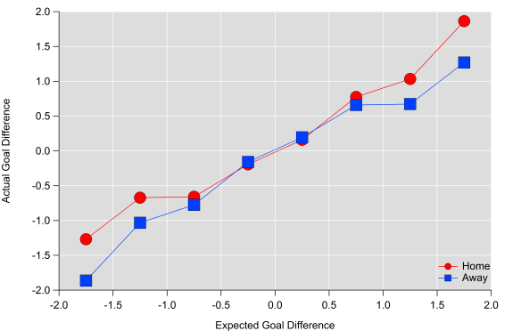
In the figure below, I’ve averaged actual goal difference from individual matches into expected goal ‘buckets’. I excluded data beyond +/- two expected goals as the sample size was quite small, although the general trends continues. Averaging like this hides a lot of details (as partially illustrated above) but I think it broadly demonstrates how the two match up.

Actual goals compared to expected goals for single matches when binned into 0.5 xG buckets.

Actual goals compared to expected goals for single matches when binned into 0.5 xG buckets.

The figure also illustrates that ‘winning’ the expected goals (xG difference greater than 1) doesn’t always mean winning the actual goal battle, particularly for the away team. James Yorke found something similar when looking at shot numbers. Home teams ‘scoring’ with a 1-1.5 xG advantage outscore their opponents around 66% of the time based on my numbers but this drops to 53% for away teams; away teams have to earn more credit than home teams in order to translate their performance into points.

What these figures do suggest though is that expected goals are a useful indicator of quality over a single match i.e. they do reflect the balance of play in a match as measured by the volume and quality of chances. Due to the often random nature of football and the many flaws of these models, we wouldn’t expect a perfect match between actual and expected goals but these results suggest that incorporating these numbers with other observations from a match is potentially a useful endeavour.

Summary

Don’t say:

Team x should have scored y goals today.

Do say:

Team x’s expected goal numbers would typically have resulted in the following…here are some observations of why that may or may not be the case today.

Recruitment by numbers: the tale of Adam and Bobby

One of the charges against analytics is that it hasn’t really demonstrated its utility, particularly in relation to recruitment. This is an argument I have some sympathy with. Having followed football analytics for over three years, I’m well-versed in the metrics that could aid decision making in football but I can appreciate that the body of work isn’t readily accessible without investing a lot of time.

Furthermore, clubs are understandably reticent about sharing the methods and processes that they follow, so successes and failures attributable to analytics are difficult to unpick from the outside.

Rather than add to the pile of analytics in football think-pieces that have sprung up recently, I thought I would try and work through how analysing and interpreting data might work in practice from the point of view of recruitment. Show, rather than tell.

While I haven’t directly worked with football clubs, I have spoken with several people who do use numbers to aid recruitment decisions within them, so I have some idea of how the process works. Data analysis is a huge part of my job as a research scientist, so I have a pretty good understanding of the utility and limits of data (my office doesn’t have air-conditioning though and I rarely use spreadsheets).

As a broad rule of thumb, public analytics (and possibly work done in private also) is generally ‘better’ at assessing attacking players, with central defenders and goalkeepers being a particular blind-spot currently. With that in mind, I’m going to focus on two attacking midfielders that Liverpool signed over the past two summers, Adam Lallana and Roberto Firmino.

The following is how I might employ some analytical tools to aid recruitment.

Initial analysis

To start with I’m going to take a broad look at their skill sets and playing style using the tools that I developed for my OptaPro Forum presentation, which can be watched here. The method uses a variety of metrics to identify different player types, which can give a quick overview of playing style and skill set. The midfielder groups isolated by the analysis are shown below.

Midfielders

Midfield sub-groups identified using the playing style tool. Each coloured circle corresponds to an individual player. Data via Opta.

I think this is a useful starting point for data analysis as it can give a quick snap shot of a player and can also be used for filtering transfer requirements. The utility of such a tool is likely dependent on how well scouted a particular league is by an individual club.

A manager, sporting director or scout could feed into the use of such a tool by providing their requirements for a new signing, which an analyst could then use to provide a short-list of different players. I know that this is one way numbers are used within clubs as the number of leagues and matches that they take an interest in outstrips the number of ‘traditional’ scouts that they employ.

As far as our examples are concerned, Lallana profiles as an attacking midfielder (no great shock) and Firmino belongs in the ‘direct’ attackers class as a result of his dribbling and shooting style (again no great shock). Broadly speaking, both players would be seen as attacking midfielders but the analysis is picking up their differing styles which are evident from watching them play.

Comparing statistical profiles

Going one step further, fairer comparisons between players can be made based upon their identified style e.g. marking down a creative midfielders for taking a low number of shots compared to a direct attacker would be unfair, given their respective roles and playing style.

Below I’ve compared their statistical output during the 2013/14 season, which is the season before Lallana signed for Liverpool and I’m going to make the possibly incorrect assumption that Firmino was someone that Liverpool were interested in that summer also. Some of the numbers (shots, chances created, throughballs, dribbles, tackles and interceptions) were included in the initial player style analysis above, while others (pass completion percentage and assists) are included as some additional context and information.

The aim here is to give an idea of the strengths, weaknesses and playing style of each player based on ranking a player against their peers. Whether a player ranks low or high on a particular metric is a ‘good’ thing or not is dependent on the statistic e.g. taking shots from outside the box isn’t necessarily a bad thing to do but you might not want to be top of the list (Andros Townsend in case you hadn’t guessed). Many will also depend on the tactical system of their team and their role within it.

The plots below are to varying degrees inspired by Ted Knutson, Steve Fenn and Florence Nightingale (Steve wrote about his ‘gauge’ graph here). There are more details on these figures at the bottom of the post*.

Lallana.

Data via Opta.

Lallana profiles as a player who is good/average at several things, with chances created seemingly being his stand-out skill here (note this is from open-play only). Firmino on the other hand is strong and even elite at several of these measures. Importantly, these are metrics that have been identified as important for attacking midfielders and they can also be linked to winning football matches.

Firmino.

Data via Opta.

Based on these initial findings, Firmino looks like an excellent addition, while Lallana is quite underwhelming. Clearly this analysis doesn’t capture many things that are better suited to video and live scouting e.g. their defensive work off the ball, how they strike a ball, their first touch etc.

At this stage of the analysis, we’ve got a reasonable idea of their playing style and how they compare to their peers. However, we’re currently lacking further context for some of these measures, so it would be prudent to examine them further using some other techniques.

Diving deeper

So far, I’ve only considered one analytical method to evaluate these players. An important thing to remember is that all methods will have their flaws and biases, so it would be wise to consider some alternatives.

For example, I’m not massively keen on ‘chances created’ as a statistic, as I can imagine multiple ways that it could be misleading. Maybe it would be a good idea then to look at some numbers that provide more context and depth to ‘creativity’, especially as this should be a primary skill of an attacking midfielder for Liverpool.

Over the past year or so, I’ve been looking at various ways of measuring the contribution and quality of player involvement in attacking situations. The most basic of these looks at the ability of a player to find his team mates in ‘dangerous’ areas, which broadly equates to the central region of the penalty area and just outside it.

Without wishing to go into too much detail, Lallana is pretty average for an attacking midfielder on these metrics, while Firmino was one of the top players in the Bundesliga.

I’m wary of writing Lallana off here as these measures focus on ‘direct’ contributions and maybe his game is about facilitating his team mates. Perhaps he is the player who makes the pass before the assist. I can look at this also using data by looking at the attacks he is involved in. Lallana doesn’t rise up the standings here either, again the quality and level of his contribution is basically average. Unfortunately, I’ve not worked up these figures for the Bundesliga, so I can’t comment on how Firmino shapes up here (I suspect he would rate highly here also).

Recommendation

Based on the methods outlined above, I would have been strongly in favour of signing Firmino as he mixes high quality creative skills with a goal threat. Obviously it is early days for Firmino at Liverpool (a grand total of 239 minutes in the league so far), so assessing whether the signing has been successful or not would be premature.

Lallana’s statistical profile is rather average, so factoring in his age and price tag, it would have seemed a stretch to consider him a worthwhile signing based on his 2013/14 season. Intriguingly, when comparing Lallana’s metrics from Southampton and those at Liverpool, there is relatively little difference between them; Liverpool seemingly got the player they purchased when examining his statistical output based on these measures.

These are my honest recommendations regarding these players based on these analytical methods that I’ve developed. Ideally I would have published something along these lines in the summer of 2014 but you’ll just have to take my word that I wasn’t keen on Lallana based on a prototype version of the comparison tool that I outlined above and nothing that I have worked on since has changed that view. Similarly, Firmino stood out as an exciting player who Liverpool could reasonably obtain.

There are many ways I would like to improve and validate these techniques and they might bear little relation to the tools used by clubs. Methods can always be developed, improved and even scraped!

Hopefully the above has given some insight into how analytics could be a part of the recruitment process.

Coda

If analytics is to play an increasing role in football, then it will need to build up sufficient cachet to justify its implementation. That is a perfectly normal sequence for new methods as they have to ‘prove’ themselves before seeing more widespread use. Analytics shouldn’t be framed as a magic bullet that will dramatically improve recruitment but if it is used well, then it could potentially help to minimise mistakes.

Nothing that I’ve outlined above is designed to supplant or reduce the role of traditional scouting methods. The idea is just to provide an additional and complementary perspective to aid decision making. I suspect that more often than not, analytical methods will come to similar conclusions regarding the relative merits of a player, which is fine as that can provide greater confidence in your decision making. If methods disagree, then they can be examined accordingly as a part of the process.

Evaluating players is not easy, whatever the method, so being able to weigh several assessments that all have their own strengths, flaws, biases and weaknesses seems prudent to me. The goal of analytics isn’t to create some perfect and objective representation of football; it is just another piece of the puzzle.

truth … is much too complicated to allow anything but approximations – John von Neumann


*I’ve done this by calculating percentile figures to give an indication of how a player compares with their peers. Values closer to 100 indicate that a player ranks highly in a particular statistic, while values closer to zero indicate they attempt or complete few of these actions compared to their peers. In these examples, Lallana and Firmino are compared with other players in the attacking midfielder, direct attacker and through-ball merchant groups. The white curved lines are spaced every ten percentiles to give a visual indication of how the player compares, with the solid shading in each segment corresponding to their percentile rank.

Square pegs for square holes: OptaPro Forum Presentation

At the recent OptaPro Forum, I was delighted to be selected to present to an audience of analysts and representatives from the football industry. I presented a technique to identify different player types using their underlying statistical performance. My idea was that this would aid player scouting by helping to find the “right fit” and avoid the “square peg for a round hole” cliché.

In the presentation, I outlined the technique that I used, along with how Dani Alves made things difficult. My vision for this technique is that the output from the analysis can serve as an additional tool for identifying potential transfer signings. Signings can be categorised according to their team role and their performance can then be compared against their peers in that style category based on the important traits of those player types.

The video of my presentation is below, so rather than repeating myself, go ahead and watch it! The slides are available here.

Each of the player types is summarised below in the figures. My plan is to build on this initial analysis by including a greater number of leagues and use more in-depth data. This is something I will be pursuing over the coming months, so watch this space.

Some of my work was featured in this article by Ben Lyttleton.

Forward player types.

Forward player types

Midfielder player types.

Midfielder player types.

Defender player types.

Defender player types.

Stats! What are they good for?

I’ve been closely following the developments in the football analytics community for close to two years now, ever since WhoScored allied themselves with the Daily Mail and suggested Xavi wasn’t so good at the football and I was directed to James Grayson’s wonderful riposte.

There has been some discussion on Twitter about the state of football analytics recently and I thought I would commit some extended thoughts on this topic to writing.

Has football analytics stalled?

Part of the Soccermetrics podcast, featuring Howard Hamilton and Zach Slaton, revolved around how football analytics as an activity has “stalled” (Howard has since attributed the “stalled” statement to Chris Anderson, although he seemingly agrees with it). Even though this wasn’t really defined, I find it difficult to comprehend the view that analytics has stalled.

Over the past two years, the community has developed a lot as far as I can see. James Grayson and Mark Taylor continue to regularly publish smart work, while new bloggers have emerged also. The StatsBomb website has brought together a great collection of analysts and thinkers on the game and they appear to be gaining traction outside of the analytics echo chamber.

In addition to this, data is increasingly finding a place in the mainstream media; Zach Slaton writes at Forbes, Sean Ingle is regularly putting numbers into his Guardian columns and there is a collection of writers contributing to the Dutch newspaper De Volkskrant. Mike Goodman is doing some fantastic work at Grantland; his piece on Manchester United this season is an all too rare example of genuine insight in the wider football media. The Numbers Game book by Chris Anderson and David Sally was also very well received.

Allied to these writing developments, a number of analytics bloggers have joined professional clubs or data organisations recently – surely it is encouraging to see smart people being brought into these environments? (One side effect of this is that some great work is lost from the public sphere though e.g. the StatDNA blog).

To me, this all seems like progress on a number of fronts.

What are we trying to achieve?

The thing that isn’t clear to me is what people in the analytics community are actually aiming for. Some are showcasing their work with the aim of getting a job in the football industry, some are hoping to make some money, while others are doing it as a hobby (*waves hand*). Whatever the motivation, the work coming out of the community is providing insights, context and discussion points and there is an audience for it even if it is considered quite niche.

Football analytics is still in its infancy and expecting widespread acceptance in the wider football community at this stage is perhaps overly ambitious. However, strides are being made; tv coverage has started looking more at shot counts over a season and heat maps of touches have made a few appearances. These are small steps undoubtedly but I doubt there is much demand for scatter plots, linear regression and statistical significance tests from tv producers. Simple and accessible tables or metrics that can be overlaid on an image of a football pitch seem to go down well with a broader audience – the great work being done on shot locations seems ripe for this as it is accessible and intuitive without resorting to complex statistical language.

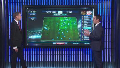
Gary Neville shows off his massive iPad.

Gary Neville shows off his massive iPad. Courtesy of thedrum.com.

However, I don’t think the media should be the be all and end all for judging the success or progress of football analytics. Fan discussion of football is increasingly found online in the form of blogs, forums and Twitter, so the media don’t have to be the gatekeepers to analytics content. Saying that, I would love to see more intelligent discussion of football in the media and I feel that analytics is well placed to contribute to that. I’d be interested to hear what it is people in the football analytics community are aiming for in the longer term.

What about the clubs?

The obvious aspect of the analytics community that I’ve omitted from the discussion so far is the role of the clubs in all this. It’s difficult to know what goes on within clubs due to their secrecy. The general impression I get is that there are analytics teams toiling away but without necessarily making an impact in decision making at the club, whether that is in terms of team analysis or in the transfer market. Manchester City are one example of a team using data for such things based on this article.

With this in mind, I was interested to listen to the Sky Sports panel discussion show featuring Chris Anderson, Damien Commoli and Sam Allardyce. Chris co-authored the excellent The Numbers Game book and brought some nuance and genuine insight to the discussion. Commoli is mates with Billy Beane. Allardyce is held up as an acolyte for football analytics at the managerial level in English football and I think this is first time I’ve really heard him speak about it. I wasn’t impressed.

Allardyce clearly takes an interest in the numbers side of the game and reeled off plenty of figures, which on the surface seemed impressive. He seemingly revels in the idea that he is some sort of visionary with his interest in analytics, repeating on several occasions how he has been using data for over ten years. He seemed particularly pleased with the “discovery” of how many clean sheets, goals and other aspects of the game were required to gain a certain number of points in the Premier League; something that many analysts could work out in their lunch hour given the appropriate data.

I would question how this analysis and many of the other nuggets he threw out are actually actionable though; much of this is just stamp-collecting and doesn’t really move things forward in terms of actually identifying what is happening at the process level on the pitch. For example, Commoli’s statistic on a team never losing when having ten or more shots on goal, which is valuable information for those footballers who don’t aim for the goal. Now it could be that they were holding back the good stuff but several of their comments suggested they don’t really understand core analytics concepts such as regression to the mean and the importance of sample size e.g. referring to Aaron Ramsey’s unsustainable early-season scoring run. I would have expected more from people purporting to be leading take up of analytics at club level.

I felt Allardyce’s comment about his “experience” being better than “maths” when discussing the relationship between money and success betrayed his actual regard for the numbers side of football. Many of the numbers he quoted seemed to be used to confirm his own ideas about the game. This is fine but I think to genuinely gain an edge using analytics, you need to see where the data takes you and make it actionable. This is hard and is something that the analytics community could do better (Paul Riley is doing great work on his blog in this area for goalkeepers). The context that analytics provides is very valuable but without identifying “why” certain patterns are observed, it is difficult to alter the process on the field.

Based on the points that Allardyce made, I have my doubts whether the clubs are any further ahead in this regard than what is done publicly by the online analytics community. If there is a place where analytics has stagnated, maybe it is the within the clubs. To my mind, they would do well to look at what is going on in the wider community and try to tap into that more.

——————————————————————————————————————–

Shorter version of this post, courtesy of Edward Monkton.

Where are we Going?

I don’t know, I thought you knew.

No I don’t know. Maybe he knows.

No, He definitely doesn’t know.

*PAUSE*

Maybe no-one knows.

*PAUSE*

Oh Well. I hope it’s nice when we get there.